Miniature Inertial Measurement Unit - IMU

IMU sensors : 1 accelerometer MMA7260 from freescale (3 axis) coupled with 2 rate gyros ADIS16080 from analog device (1 axis each)

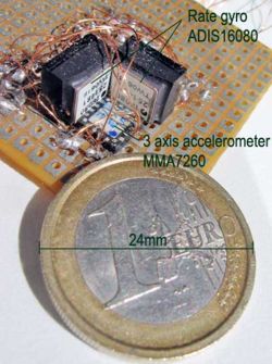
A DIY Miniature Inertial Measurement Unit implemented on a dsPIC with a rapid prototyping tool.

An Inertial Measurement Unit is based on inertial sensors to estimate its absolute angle in space also called atitude.

All files including simulink model, matlab script and data files (.mat) can be downloaded : see the Download section.

Introduction

The micro-Inertial Measurement Unit (IMU) presented here estimates its atitude around two rotation angles only: pitch and roll. The three principal components are:

• 2 one axis MEMS rate gyro measuring roll and pitch speed rate
• 1 tri axial MEMS accelerometer measuring both the IMU acceleration and the gravity
• 1 dsPIC (30f or 33f) or 1 PIC24

The atitude of the IMU system is estimated using information from the rate gyros and the accelerometers.

After a quick description of the angle estimation using accelerometers or gyro, this document describe the electronics board and explain how logging data through the UART port of the PC. Then, the document presents the different estimation methods that fuse data from gyros and accelerometers to retrieve the atitude of the IMU system:

• Complementary filter
• non-adaptative Kalman filter

Simulink simulation of these two methods, relying on real data previously logged, provide an easy way to tune each method, and to compare their efficiency. Once tuned, one method is implemented in the embedded PIC or dsPIC microcontroller in no time with the one push button method: the rapid prototyping tool described on this website (dsPIC blockset for Simulink).

Problems of estimating angles from inertial sensors

Estimating angles from rate gyro

A rate gyro measures its angular speed rate. Low noise and high precision of theses MEMS sensors are very good. Thus, integrating the value of the rate gyro over time provide a good estimation of the angular displacement. Provided the initial position of the system is known and the sensor is ideal, the integration would provides the correct angular orientation. The integration function also acts as a low pass filter. The sensor noise, which is already low, is even lowered by this integration.

Unfortunately, the rate gyro sensor is not ideal. Integrating the rate gyro also integrate its DC value. The integration of any error induced an unrecoverable bias on the estimated angle. As this DC value drifts slowly over time, it is not possible to cancel it by subtracting to the gyro output its DC offset value. Thus, a typically integration of a gyro would result in an angle drift of about 1° within one minute (depending on the rate gyro used!). It is necessary to use another sensor so as to recover the bias introduced by the integration of errors.

• <Tex>\Theta</Tex> the absolute pitch angle and q the pitch angular rate.

<Tex>\hat \Theta(t) = \int_{t_0}^t{q(t) dt}+\Theta(t_0)</Tex>

• <Tex>\Phi</Tex> the absolute roll angle and p the roll angular rate.

<Tex>\hat \Phi(t) = \int_{t_0}^t{p(t) dt} + \Phi(t_0)</Tex>

Estimating angles from accelerometers

Accelerometers sense the both the gravity vertical acceleration vector (9.81m/s^2) added to the acceleration of the sensor itself. Accelerometers are usually quite noisy and needs to be filtered. The acceleration of a system could in many case considered as small compared to the gravity acceleration value. If the system is considered as not accelerating (Hovering helicopters, flying gliders in stable straight flight...), it is possible to extract the pitch and roll absolute angle using the measured gravity vector.

• ax the acceleration measured with the accelerometer on the x axis (longitudinal)
• ay the acceleration measured with the accelerometer on the y axis (lateral)
• az the acceleration measured with the accelerometer on the z axis (vertical)

Using the acceleration vector (i.e. gravity) measured with the accelerometers, we get the <Tex>\Theta</Tex> and <Tex>\Phi</Tex> angles :

• <Tex>\hat \Theta= \arctan \left( \frac{a_z}{a_x} \right)</Tex>
• <Tex>\hat \Phi = \arctan \left( \frac{a_z}{a_y} \right)</Tex>

Note than when the axis az and ay are in the horizontal plane, the result is undefined. But pitch or roll angle is not defined as well (think of a plane which has its nose in the sky, perpendicular to the horizontal. Its absolute roll angle is undefined). Absolute calibration of the accelerometers gain is not necessary because a rapport is calculated. The only point to care about is the offset of the three axes and the gain that must be the same for all three axes.

However, the first weakness of the angle estimated from accelerometers is its sensibility to the acceleration of the system. In others words, the estimated angle is biased whenever the system accelerates. The second weakness is the noisy result due to the accelerometers sensors.

Estimating angles from both rate gyro and Accelerometers

Angle estimation from either a rate gyro or accelerometers only do not provide good results. The characteristics of these two types of sensors are complementary:

• Gyros provide a clean estimation of angle in dynamic situation on a short range time
• Accelerometers provide a noisy but absolute angle reference in static situation

It is therefore possible make a data fusion algorithm so as to couple the static reference angle computed from the Accelerometers with the dynamic angle variation estimation from the rate gyro. The fusing algorithm tuning takes into account the dynamic of the system. If the system is often accelerating wigh high acceleration compared to the gravity (9,8m/s^2), the estimated angle will rely mostly on the rate gyro so as to remove the errors introduced by the acceleration measurement.

Embedded Electronics

This IMU use three MEMS sensors : One Three axial accelerometer (analog) and two one axis rate gyro with SPI interface. The 3 axes accelerometer MMA7260QT is powered by the 2.5V analog output reference created by the 'Y axis' rate gyro

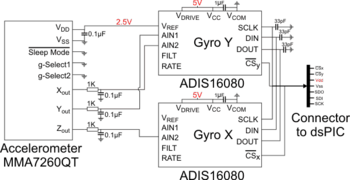
The Embedded IMU Schematic is equipped with 1 accelerometer (3 axis) coupled with 2 rate gyro (1 axis each).

One of the gyro supplies the 2.5V alimentation required by the accelerometer. Each gyro has two analog input pin connected to its internal ADC. Thus, the two gyros convert the three analog values of ax, ay, and az from the accelerometer. The IMU transmit the 5 data (3 acceleration + 2 rate gyros) to the microcontroller through a SPI bus.

The dsPIC used (dsPIC 30f4012) is equipped with a 10Mhz quartz. This quartz frequency allows using the UART at 115200bps which is the max baud rate available on most personal computers (Serial port's limitation).

Log raw data from sensor for simulink simulation

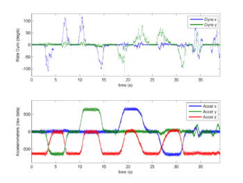
Data from the inertial sensors are logged with matlab. Theses real data feeds a simulink model giving the possibility to develop/debug/compare different angle estimation algorithm.

All sensor data are received through the SPI peripheral of the dsPIC. Data are received from the two gyros using the SPI Input/Output interrupt driven block. The code generated by this block use interrupt to constantly pool the two gyros and obtain the data. The output of the block is the most recent data received (for each requested data).

Data are transmitted through the UART peripheral. We have the following constraints:

• model time-step is 1ms
• UART speed rate is 115200bps
• 5 values of 12 bits resolution must be transmitted

Two methods to log datas are explained: The first logging method use the Tx Output Multiplexed for Matlab-Labview block. The other method use the Tx Output block. Both logging method use the graphical matlab interface developed: Interface Tx-Matlab

Using the UART Tx Output Multiplexed for Matlab-Labview block

IMU_dsPIC_30f4012_TestElectronics Simulink model: Once this model is compiled, the dsPIC (30f4012) transmit the values from the X, Y and Z axis of the accelerometer, and the Y and X axis of the rate gyro. Data are sent to Matlab (or labview) through the UART at 115200bps with the Tx Output Multiplexed for Matlab-Labview block. All data cannot be send ; there will be missing data thus this model is usefull to check every component is working only.

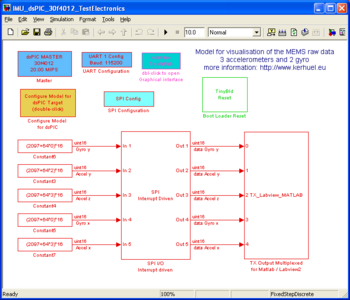
The model IMU_LogData is compiled and the generated .hex file is loaded into the dsPIC (using the bootloader tinybld). The model samples the data at 1kHz, corresponding to the time-step of 1ms. During 1ms, the UART can send 11,52 Bytes when configured at 115200 bps (taking into account the start and stop bits). We log 5 int16 data that correspond to 10 bytes. The multiplexing protocol of the Tx Output Multiplexed for Matlab-Labview block.]] adds one byte for each variable sent. Thus, the model sends 15 bytes at each time step. Because the model sends more than 11 data by time-step, some data will be lost. The Intelligent Spreading option will spread the lost over all data allowing to view all data on the graph (If not checked, the two last data may never be sent).

Because of the lost of some data, it is OK for plotting data and allows checking than all components are working. It is Not OK to use these data as input data in a Simulink simulation! (You may however interpolate the data…)

The data that get out from the Tx Output Multiplexed for Matlab-Labview block are the sensor raw data. It is 16 bits data but only the 12 lower bits contains the measured value.

The dsPIC is connected to the PC COM port (using an equivalent to Max232 component for level translation) and data are logged using the graphical user interface. The following lines are typed at the maltab prompt to save data into a .mat file:

 >> [R T] = padr(Rn,1,t_Rn);     % remove NaN values
 >> datas = [T R]';
 >> save mydatafile datas;

Keep in mind than missing data on columns [2 3 4 5] are stuffed with their previous non missing value. Missing data on column 1 suppressed the time step. In other word, data is corrupted and should not feed a simulink simulation. If we decided to log 3 datas only (2 accelerometers and 1 gyro), all data would have been received (9 bytes sent each time step). The resulting file could feed a simulink simulation. Another method described below allows logging all the 5 values at 1kHz without missing data!

padr is a command from the blockset. It allows removing the NaN from the Rn matrix. The resulting R matrix is transposed and time is added in its first line. The time T which is a modified copy of t_Rn is not accurate since it is estimated by the time at which values are received. We know that the data are sent at a 1Khz frequency so we can redefine the time of the AxelX_GyroY_AxelZ matrix before saving it into the AxelX_GyroY_AxelZ3.mat file.

Using the UART Tx Output block

IMU_dsPIC_30f4012_LogData_Raw Simulink model: Once this model is compiled, the dsPIC (30f4012) transmit the raw values from the MEMs sensors. Data are sent to Matlab (or labview) through the UART at 115200bps with the Tx Output block. The UART buffer do not overflow with this mode, because 9 bytes are sent and the 115200bpd UART speed allow to send 11,52 bytes in one 1ms time-step. Thus all data are successfully transmitted to matlab. Logged data can feed a simulink simulation.

The UART at 115200 can transmit only 11,52 data within a 1ms time-step. Thus, the simulink model implemented on the dsPIC must transmit less or equal 11 datas to be sure that there will be no data lost.

5 data with a 12 bits length must be transmitted. The solution described code each data into 2 data bytes (16 bits). One signature byte with the value 55 sent first is sent before the 10 bytes frame to provide a synchronization reference. This signature byte may also be used to check that no data were lost (checking that 10 bytes are present between two 55 values).

From the matlab GUI interface >> rs232gui, data received are no more multiplexed with the Tx Output Multiplexed for Matlab-Labview block. The demultiplexing algorithm is switched off by clicking on the RAW button of the interface. The script embedded in the rs232gui interface should be cleared. The R vector is the raw data received by the Serial port of the computer. The R vector is saved (files Rawdatas*.mat). The script Extract_RawDatas.m load the saved R vector and extract the 5 values. Part of the script is shows below.

Raw data from the sensor. On this experiment, the IMU box were rotated by 90 degrees with interval of about 5s. File RawDatas_Dynamic_Calibration_40se.mat plotted using the script Extract_RawDatas. Theses raw data are saved in a .mat file and are used to feed a simulink simulation.

R = reshape(R,11,n); % reshape : from vector to a matrix of 11 column
idxError = find(R(1,:) ~= 55)  % Check data integrity
if ~isempty(idxError)
    error('Data corrupted')
end
 
%% Reconstruct Raw data as received through the SPI bus
RawGyro_Y = R(2,:)*2^8 + R(3,:);
RawAccel_Y = R(4,:)*2^8 + R(5,:);
RawAccel_Z = R(6,:)*2^8 + R(7,:);
RawGyro_X = R(8,:)*2^8 + R(9,:);
RawAccel_X = R(10,:)*2^8 + R(11,:);
T = [0:.001:(length(RawGyro_Y)-1)*.001];

The simulink model embedded on the dsPIC send data when the value variable60 is different from 0. This variable is changed throught the UART. When receiving values [60 x], the embedded simulink model load the value x into the variable variable60. The values [60 x] can be sent using the rs232gui interface. The Simulink model decreases automatically this variable by 1 each second. This makes the user able to log data during a predefined time.

Simulation based on real data

Simulation of an IMU based on real logged data. Complementary Filter and a non-adaptative Kalman Filter are simulated and compared.

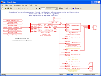
The model IMU_Simulation.mdl uses the logged data stored in .mat files. These data are used to design, and simulate algorithm to estimate angles. Because we are using real data, the input of the simulation has precisely the right properties (noise, bias...). The data stored are exactly the same data read at the output of sensors. Once the simulation provide optimal result, it is possible to implement the simulation as is in the PIC/dsPIC.

The raw data feeds a block called Sensor Calibration. This block removes bias of rate gyro and accelerometers.

Rate gyro gain is also set. On the electronic board, the gain of the gyro does not comply with the datasheet value. The Y gyro can measure a range of ± 524°/s with a resolution of 0.26°/s. The X gyro can measure a range of ± 188°/s with a resolution of 0.09°/s. The datasheet give an angular speed rate of ±80°/s with a resolution of 0.039°/s.

Because we use the arctan function, the accelerometer axes do not need to be scaled.

Complementary Filter

Complementary Filter for IMU angle estimation

A complementary filter combines the two estimations. High frequency part of the angle estimated from the rate gyro is added to the low frequency part of the angle estimated with the accelerometer. Thus, the low drift of the estimated angle from the gyro is filtered and only high frequency estimated angle from the gyro is used. The low frequency part of the angle estimated rely on the angle estimated using the accelerometer. The high frequency of the angle is estimated with the gyro which provide a fast and accurate information but which cannot be integrated due to the accumulation of the bias error.

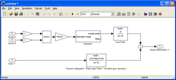
The upper part of the complementary filter block estimates the Y axis angle computing the arctan of the X and Z accelerometers values. The lower part of the complementary filter blocks estimates the Y axis angle integrating the Y rate gyro. The dynamic of the gyro (low pass filter) is compensated for. The rate gyro is also high pass filtered to remove most of the DC part. The complementary filter, two first order filter (high pass and low pass) with cut off frequency at 0,08Hz. The final estimation of the angle is the addition of the resulting values from theses two filters. The result is presented in pink on the lower part of the following figure.

Top curves : The X (yellow) and Z (cyan) accelerometers raw data with the Y axis rate gyro (pink). The y scale is the raw numerical value as read from the Gyro-SPI bus. The x scale is time (simulation duration is 33,32s). The three bottom curves are the simulated estimation of the angle (Y axis) using three different methods. The yellow curve is the estimated angle from the X and Z accelerometers, sensing the gravity. The cyan curve is the estimated angle, integrated from the Y rate gyro. The pink curve is the estimated angle estimated with the complementary filter that fusion the relevant information from both the Y rate gyro and the X-Z accelerometer

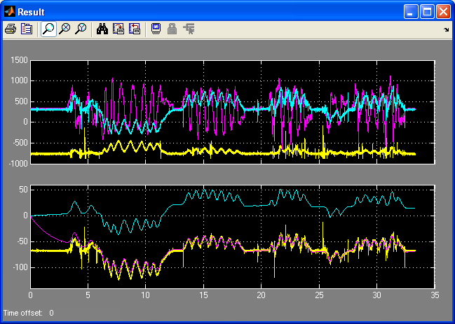
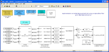
Complementary Filter running on dsPIC

This model implements the complementary filter on the dsPIC and sends the result to matlab. It has the same behaviors as the simulated filter.

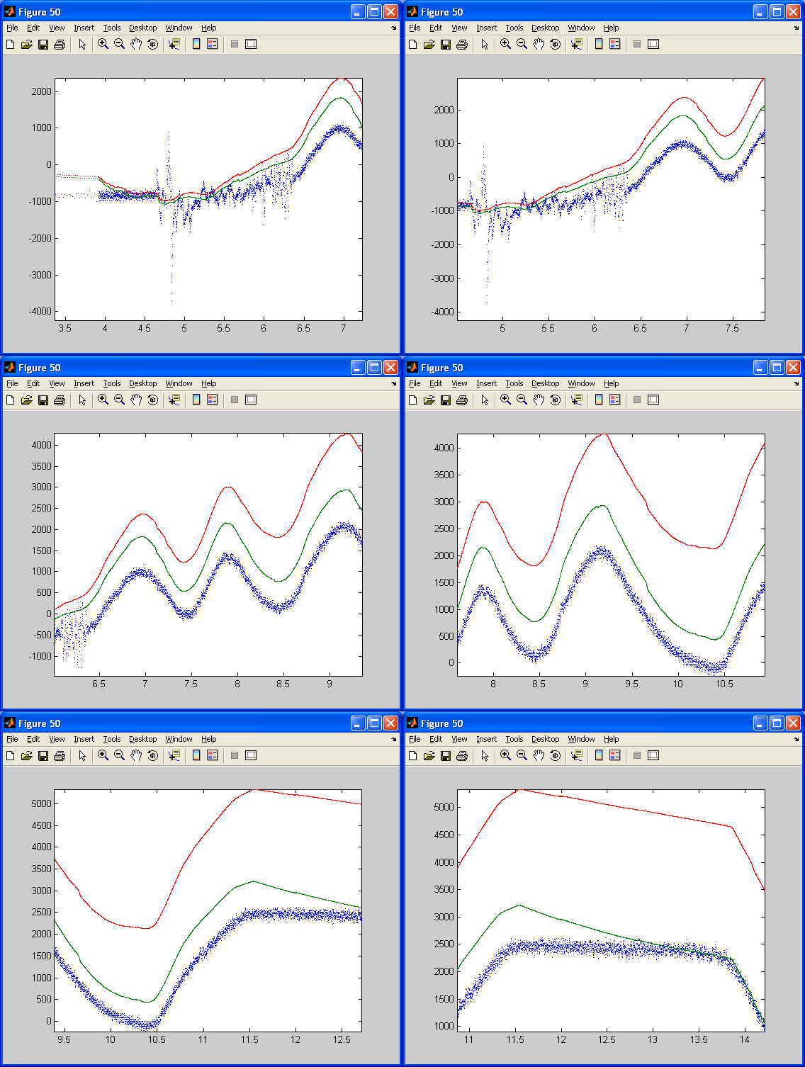
To design the filter for the dsPIC, the two precedent models are mixed up. The filter is inserted by copy-past into the first model used to log data. Data logged in real time from the complementary filter implemented on the dsPIC (30f4012 running at 10MHz). X axis : time in second. Y axis : angle multiplied by 100 (see model) The blue curve is the estimated angle from the X and Z accelerometers, resolving the gravity vector. The red curve is the estimated angle integrated from the Y rate gyro. The green curve is the angle estimated through the complementary filter that fusion the relevant information from both the Y axis rate gyro and the X and Z accelerometers.

The estimated angle using accelerometers (blue curve) is quite noisy. However, it steady value is correct. The estimated angle relying on the integration of the gyro is clean but drift (red curve). Note that the dsPIC has just been switch on and the High pass filter of the pseudo integrator of the gyro has not yet removed the remaining DC bias of the gyro. The DC bias of the Gyro has probably changed due to non constant temperature in my house. (I do not have a clim in my tiny room which is in a roof in Marseille! ). Thus, the gyro integrated angle is slowing drifting away from its real value. The green curves that use both data is clean and drift free. Its dynamics is as fast as the gyro dynamic. Note that at the beginning, the High pass filter (with a higher bandwidth than the gyro pseudo-integrator high pass filter) has not yet removed the gyro bias. However, at the end of the animation (11 seconds long: from 3, 5 to 14, 5), both curves (blue and green) are merging as in the simulation.

Remarks about complementary filter

The high pass filter, the inverted rate gyro dynamic and the integrator are merged into one transfer function.

All calculation is done in double data type or single data type. Theses float data slow down the calculation and use a large amount of memory. It is quite powerful with the help of simulink to build a fixed point complementary filter. Thus, next step is to go back to the simulation model and to design a fixed point complementary filter! (Using the matlab fixed point toolbox)

Non adaptative Kalman Filter

The non adaptative Kalman filter track the rate gyro bias and estimate the angle by integrating the unbiased gyro.

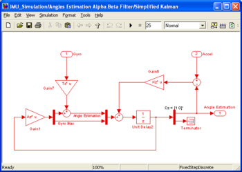
The non adaptative Kalman Filter (Also called Alpha Beta Filter) track the gyro bias using information from the accelerometers, then estimate the angle by integrating the unbiased gyro.

to be continued...

Non adaptative Kalman Filter running on dsPIC

explanations comming soon. have a look on model files...

Conclusion

Programming dsPIC or PIC24 becomes exciting and fun with this toolbox. You do not have to waste your time with configuration of the dsPIC peripherals! Focus only on simulink simulation, Real time Workshop capabilities, and on fixed point optimization.

Download

IMU_for_dsPIC.zip : All Simulink and Matlab file used with data logged.

The demo version of the blockset could compile model with up to 6 I/O pins. The Simulink model presented could not be compiled as is with the demo version of the blockset because SPI bus use 5 pins and UART uses 2 pins. Removing the UART blocks, makes possible compiling theses models. Adding for example one PWM output may give the possibility to get the result for one angle.

List of files:

• Simulink models
  • IMU_dsPIC_30f4012_TestElectronics.mdl
  • IMU_dsPIC_30f4012_LogData_Raw.mdl
  • IMU_Simulation.mdl
  • IMU_dsPIC_30f4012_ComplementaryFilter_20Mips.mdl
  • IMU_dsPIC_30f4012_AlphaBetaFilter_20Mips.mdl
• M script
  • Extract_RawDatas.m
  • Script_Kalman.m
  • RealTimeVisualisationScript.m
• Mat files
  • RawDatas_*.mat : Raw data received from the dsPIC
• mat files to feed simulink model file IMU_Simulation.mdl
  • Simulink_Dynamic_Calibration.mat
  • Simulink_Dynamic_Calibration2.mat
  • Simulink_Dynamic_Calibration3.mat
  • Simulink_Static.mat
  • Simulink_Static_60s.mat

On-going projects

I am planning to use this IMU in an autopilote for remote controlled glider ( as previous project described on my french website : http://lubink.free.fr)

Point to clarify, error, remarks ? Please, leave your comment on the forum !